Welcome to cse102-notes’s documentation!

Introduction

What is an Algorithm?

• Computational processes for solving problems (i.e. a formal procedure followable by a computer)

• Foundational subject in CS

  • Even most simple operations, like addition: how do you compute the binary representation of X + Y?

What does Analysis mean?

• Proving algorithms correct (every input has the correct output)

• Working out time/memory requirements to solve problems of a given size

• Designing algorithms for new problems

  • Toolkit of general techniques for designing algorithms (e.g. divide-and-conquer, dynamic programming)

Example

The Convex Hull Problem

Input: a set of points in the 2D plane (as a set of (x, y) coords)

Output: the convex hull (the smallest convex polygon containing all the points)

One algorithm used to solve this problem is “gift wrapping”:

find the lowest point (min y-coord)  # top, leftmost, etc also work
rotate a ray going directly east of the point CCW until it hits a point
repeat until the ray returns to the start

You can find the “first point CCW” by calculating the angle from a given point to all other points, and taking the lowest:

How long does this take?

For a worst case, \(O(n^2)\) - you calculate N angles to each other point from each of the N points.

However, there is a faster divide-and-conquer algorithm:

find convex hull for the left/right halves of the set
combine them by the tangents of each polygon

Algorithms

a computational procedure to solve a problem

Problem

a mapping or relation from inputs to outputs

• Input: an instance of the problem

  • e.g. an input might be a list of points in the convex hull problem

  • the encoding of the instance into a binary sequence is important - solving for lists of pairs of numbers is different than solving for strings

• Output: solution to the problem instance

  • e.g. a list of points making up the convex hull, in order

  • there can be multiple valid solutions for some problem instances, e.g. sorting

Key property of an algorithm for problem P: for any instance of P, running the algorithm on the instance will cause it to eventually terminate and return a corresponding solution

If an algorithm does so, it is called correct.

To measure the time for an algorithm to execute, we need to define “computational procedure”:

Computational Procedure

the RAM model

Idea: algorithm = program running on an abstract computer, e.g. Turing Machine (CSE 103)

The RAM model is an abstract computer that is more complex than TMs but closer to a real computer.

RAM Model

• registers

  • store some finite amount of finite-precision data (e.g. ints or floats)

• random access memory (RAM)

  • stores data like registers, but with infinitely many addresses

  • can look up the value at any address in constant time

• program

  • a sequence of instructions that dictate how to access RAM, put them into registers, operate on them, then write back to RAM

  • e.g. load value from RAM/store into RAM

  • arithmetic, e.g. add r3 r1 r2

  • conditional branching, e.g. “if r1 has a positive value goto instruction 7”

So, an algorithm is a program running on a RAM machine - in practice, we define algoritms using pseudocode, and each line of pseudocode might correspond to multiple RAM machine instructions.

Runtime

The runtime of an algorithm (on a particular input) is then the number of executed instructions in the RAM machine.

To measure how efficient an algorithm is on all inputs, we use the worst case runtime for all inputs of a given size.

For a given problem, define some measure n of the size of an instance (e.g. how many points in the convex hull input set, number of elements in a list, number of bits to encode input). Then the worst case runtime of an algorithm is a function f(n) = the maximum runtime of the algorithm on inputs of size n.

Ex. The convex hull gift wrapping algorithm has a worst-case runtime of roughly \(n^2\), where n is the # of points.

Note

Pseudocode may not be sufficient for runtime analysis (but fine for describing the algorithm) - for example, each of the lines below is not a constant time operation

Ex. Sorting an array by brute force

• Input: an array of integers [A[0]..A[n-1]]

For all possible permutations B of A:   # n!
    If B is in increasing order:        # O(n)
        Return B

In total, this algorithm runs on the order of \(n! \cdot n\) time (worst case).

“Efficient”

For us, “efficient” means polynomial time - i.e. the worst case runtime of the algorithm is bounded above by some polynomial in the size of the input instance.

E.g. the convex hull algorithm was bounded by \(cn^2\) for some \(c\), but the brute force sorting algorithm can take \(> n!\) steps, so it is not polynomial time.

Note

e.g. “bounded above”: \(f(n) = 2n^2+3n+\log n \leq 6n^2\)

i.e. there exists a polynomial that is greater than the function for any n.

e.g. \(2^n\) is not bounded above by any polynomial

In practice, if there is a polynomial time algorithm for a problem, there is usually one with a small exponent and coefficients (but there are exceptions).

Polynomial-time algorithms are closed under composition, i.e. if you call a poly-time algorithm as a subroutine polynomially many times, the resulting algorithm is still poly-time.

Asymptotic Notation

a notation to express how quickly a function grows for large n

Big-O

upper bound

\(f(n) = O(g(n))\) iff \(\exists n_0\) s.t. for all \(n \geq n_0, f(n) \leq cg(n)\) where \(c\) is some constant

f is asymptotically bounded above by some multiple of g.

Ex.

• \(5n = O(n)\)

• \(5n + \log n = O(n)\)

• \(n^5 + 3n^2 \neq O(n^4)\) since for any constant c, \(n^5\) is eventually larger than \(cn^4\)

• \(n^5 + 3n^2 = O(n^5) = O(n^6)\)

Note

\(O(g)\) gives an upper bound, but not necessarily the tightest such bound.

Big-\(\Omega\)

lower bound

\(f(n) = \Omega(g(n))\) if \(\exists c > 0, n_0\) s.t. \(\forall n \geq n_0, f(n) \geq cg(n)\)

Ex.

• \(5n = \Omega(n)\)

• \(5n+2 = \Omega(n)\)

• \(n^2 = \Omega(n)\)

Big-\(\Theta\)

tight bound

\(f(n) = \Theta(g(n))\) if \(f(n) = O(g(n))\) and \(f(n) = \Omega(g(n))\)

• if \(f(n) = \Theta(n)\), it is linear time

• \(\log n = O(n)\) but \(\neq \Theta(n)\)

• \(5n^2+3n = \Theta(n^2)\)

Examples

As example done in class, \(\log_{10}(n)\) is:

• \(\Theta(\log_2(n))\)

  • Because \(\log_{10}(n)=\frac{\log_2(n)}{\log_2(10)} = c\log_2(n)\) for some c

• NOT \(\Theta(n)\)

  • need \(\log_{10}(n) \geq cn\) for some \(c > 0\) for some sufficiently large n, which does not hold

  • so \(\log_{10}(n) \neq \Omega(n)\)

• \(O(n^2)\)

• \(\Omega(1)\)

  • \(\log_{10}(n) \geq c \cdot 1\) for some c

• \(\Theta(2\log_{10}(n))\)

  • You can set \(c = \frac{1}{2}\)

Some particular growth rates:

• Constant time: \(\Theta(1)\) (not growing with n)

  • e.g. looking up an element at a given array index

• Logarithmic time: \(\Theta(\log n)\) (base does not matter)

  • e.g. binary search

• Linear time: \(\Theta(n)\)

  • e.g. finding the largest element in an unsorted array

• Quadratic time: \(\Theta(n^2)\)

• Exponential time: \(\Theta(2^n), \Theta(1.5^n), \Theta(c^n), c > 1\)

  • e.g. brute-force algorithms

Recurrence

When analyzing the runtime of a recursive algorithm, you can write the total runtime in terms of the runtimes of the recursive calls, creating a recurrence relation.

E.g. the divide-and-conquer convex hull algorithm, with 3 main steps:

Split points into left and right halves                 # O(n)
Recursively find the convex hulls of each half          # 2T(n/2)
Merge the 2 hulls into a single one by adding tangents  # O(n)

So in total:

\[\begin{split}T(n) & =O(n)+2T(\frac{n}{2})+O(n) \\ & =2T(\frac{n}{2})+O(n)\end{split}\]

Note: A base case is required for recurrences; problem-specific (for convex-hull \(n \leq 3\) is the base case)

Solving

Recursion Tree

e.g. \(T(n)=2T(\frac{n}{2})+O(n)\)

Solving for the max depth of the base case: \(\frac{n}{2^d}\leq 3 \to 2^d \geq \frac{n}{3} \to d \geq \log_2(\frac{n}{3}) = \log_2(n) - \log_2(3) = \Theta(\log n)\)

In conclusion, the work at each level is \(\Theta(n)\), with \(\Theta(\log n)\) levels, so the total runtime is \(\Theta(n \log n)\).

The recursion tree is used informally to guess the asymptotic solution of a recurrence, but it does not prove the solution works.

Induction/Substitution

Solve for a guess using some other method (e.g. recurrence tree), then use subtitution to prove.

e.g. \(T(n)=2T(n/2)+O(n)\)

• guess that \(T(n)=O(n \log n)\)

• need to prove \(\exists n_0, c > 0\) s.t. \(\forall n \geq n_0, T(n) \leq c n \log n\).

Fix \(n_0\) and \(c\), and prove \(T(n)\leq cn \log n\) for \(n \geq n_0\) by induction on n

• Base case (\(n = n_0\)): Need \(T(n_0) \leq cn_0 \log n_0\)

  • Take \(n_0 > 1\), then pick c large enough to satisfy the inequality

• Inductive case: Assume \(T(m) \leq cm \log m\) for all \(m < n\)

  • then \(T(n) = 2T(n/2)+O(n)\)

  • since \(n/2 < n\), \(T(n/2)\leq c \frac{n}{2} \log \frac{n}{2}\) (by IH)

  • \(T(n) \leq \frac{2cn}{2} \log \frac{n}{2} + dn\) (for some constant d)

  • \(T(n) \leq cn (\log \frac{n}{2}) + dn\)

  • \(= cn (\log n - \log 2) + dn\)

  • \(= cn \log n + n (d -c \log 2)\)

  • \(\leq cn \log n\) if \(c \geq \frac{d}{\log 2}\)

  • This establishes the inductive hypothesis at n.

• By induction, \(T(n) \leq cn \log n\) for all \(n \geq n_0\).

If you wanted to prove \(\Theta(n)\), the proof would look similar to the proof above, but with the \(\leq\) and \(\geq\) reversed to prove \(\Omega(n)\).

Master Theorem

For recurrences of the form \(T(n) = aT(n/b) + f(n)\), we can use the master theorem for divide-and-conquer recurrences. (not proved in class - proof by recursion trees in CLRS)

Thm: If \(T(n)\) satisfies a recurrence \(T(n) = aT(n/b) + f(n)\) where \(a \geq 1, b > 1\), or the same recurrence with either \(T(\lfloor n/b \rfloor)\) or \(T(\lceil n/b \rceil)\), then defining \(c = \log_b a\), we have:

1. If \(f(n) = O(n^{c-\epsilon})\) for some \(\epsilon > 0\), \(T(n) = \Theta(n^c)\)

2. If \(f(n) = \Theta(n^c)\), \(T(n) = \Theta(n^c \log n)\)

3. If \(f(n) = \Omega(n^{c+\epsilon})\) for some \(\epsilon > 0\) and \(af(n/b) \leq df(n)\) for some \(d < 1\) and sufficiently large n, \(T(n) = \Theta(f(n))\)

Examples

• \(T(n) = 9T(n/3)+n\)

  • \(c = \log_3 9 = 2\)

  • Case 1: \(n = O(n^{2-\epsilon})\)

  • so \(T(n) = \Theta(n^2)\)

• \(T(n) = T(2n/3)+1\)

  • \(c = \log_{3/2} 1 = 0\)

  • Case 2: \(1 = \Theta(n^0) = \Theta(1)\)

  • so \(T(n) = \Theta(\log n)\)

• \(T(n) = 3T(n/4)+n^2\)

  • \(c = \log_4 3 < 1\)

  • Case 3: \(n^2 = \Omega(n^{c+1})\) (\(\epsilon = 1, c + 1 < 2\))

  • check: is \(3(n/4)^2 \leq dn^2\) for some d?

    • \(\frac{3}{16}n^2 \leq dn^2\) for \(d=\frac{3}{16}<1\)

  • so \(T(n)=\Theta(n^2)\)

• \(T(n)=4T(n/2)+3n^2\)

  • \(c=\log_2 4 = 2\)

  • Case 2: \(3n^2=\Theta(n^2)\)

  • so \(T(n)=\Theta(n^2 \log n)\)

There is a generalization of the master theorem for differently-sized methods: the Akra-Bazzi method (not in this class)

Divide-and-Conquer Algorithms

general paradigm used by many algorithms

1. Divide the problem into subproblems

2. Conquer (solve) each subproblem with a recursive call

3. Combine the subproblem solution into an overall solution

This approach is helpful when it isn’t clear how to solve a large problem directly, but you can rewrite it in terms of smaller problems. Coming up with a way to divide/conquer may be easier than solving the whole problem.

Mergesort

e.g. Mergesort: sort a list by recursively sorting two halves - the hard part is merging two sorted lists.

define merge(B, C):

B = [3, 5, 5, 7]  # example data
C = [1, 4, 6]
D = []

look at the first element of each list
pop the smaller and append it to D (or use a pointer to track where in each list you are, etc)

B = [3, 5, 5, 7]
C = [4, 6]
D = [1]

repeat until at least one list is empty

B = [5, 5, 7]
C = [4, 6]
D = [1, 3]

B = [5, 5, 7]
C = [6]
D = [1, 3, 4]

B = [5, 7]
C = [6]
D = [1, 3, 4, 5]

B = [7]
C = [6]
D = [1, 3, 4, 5, 5]

B = [7]
C = []
D = [1, 3, 4, 5, 5, 6]

append the rest of the non-empty list to D

The runtime of the merge operation is linear, i.e. \(\Theta(|B|+|C|)\)

Now we can define mergesort:

def mergesort(A[0..n-1]):
    if n <= 1:
        return A
    mid = floor(n/2)
    left = mergesort(A[0..mid-1])
    right = mergesort(A[mid..n-1])
    return merge(left, right)

The runtime is covered in section (a/n: I didn’t attend, but it’s \(\Theta(n \log n)\)).

Proving Mergesort

How do we prove its correctness? For D/C, induction - assume the recursive calls are correct, and prove correctness given that.

Need to prove that for any list A[0..n-1], mergesort(A) is a sorted permutation of A. Prove by (strong) induction on n.

• Base Case: \(n \leq 1\)

  • Then mergesort(A) = A

  • but A is already sorted.

• Inductive Case: Take any \(n > 1\), and assume the inductive hypothesis holds for all \(k < n\).

  • Then \(m = \lfloor n/2 \rfloor < n\)

  • the length of the left half is \(m\)

  • the length of the right half is \((n-1)-m+1=n-m=n-\lfloor n/2 \rfloor=\lceil n/2 \rceil < n\)

  • so B = mergesort(A[0..m-1]) is a sorted permutation of A (by IH)

  • similarly, C = mergesort(A[m..n-1]) is a sorted permutation of A

  • since B and C are sorted, by correctness of merge(), D is a sorted permutation of B concatenated with C

  • since B is a permutation of the A[0..m-1] and C is a permutation of A[m..n-1], D is a permutation of A[0..n-1]

Designing

Two questions:

• How do you divide the problem into subproblems?

• How do you combine the subproblem solutions to get an overall solution?

Integer Multiplication

Given integers x, y, compute x * y.

Note

On a RAM machine, you can only multiply numbers in constant time if they fit in registers; otherwise you need an algorithm.

Elementary Multiplication

    37
x  114
------
   148
   370
+ 3700
------
  4218

If x and y have n digits each, how long does this algorithm take? Each iteration takes linear time, and there are linearly-many iterations, so \(\Theta(n^2)\) in total.

Divide-and-Conquer

Simple idea: split the digits in half, e.g. \(4216 = 42 * 10^2 + 16\)

In general, given an \(\leq n\)-digit integer x, \(x = x_1*10^{n/2}+x_0\) (assuming n is a power of 2).

Likewise, we can write \(y = y_1*10^{n/2}+y_0\).

Then:

\[\begin{split}xy & = (x_1*10^{n/2}+x_0) * (y_1*10^{n/2}+y_0) \\ & = x_1y_1*10^n + (x_1y_0+x_0y_1)*10^{n/2} + x_0y_0\end{split}\]

This results in 4 multiplications of \(n/2\)-digit numbers: do these recursively. The multiplications by \(10^n\) are just adding zeros, and the additions can be done in linear time.

So, as there are 4 recursive calls, we have:

\[T(n) = 4T(n/2) + \Theta(n)\]

By the master theorem, this results in \(T(n) = \Theta(n^2)\) - which is not faster than the naive algorithm.

Gotta Go Fast

Let’s look at

\[\begin{split}z & = (x_1+x_0)(y_1+y_0) \\ & = x_1y_1 + (x_1y_0 + x_0y_1) + x_0y_0\end{split}\]

Then \(x_1y_0 + x_0y_1 = z - x_1y_1 - x_0y_0\).

So with only 3 multiplications, we can get all 3 terms we need for the algorithm:

• \(x_1y_1\)

• \(x_0y_0\)

• \((x_1+x_0)(y_1+y_0) = z\)

and you can substitute into the earlier equation \(xy = x_1y_1*10^n + (z - x_1y_1 - x_0y_0)*10^{n/2} + x_0y_0\) to obtain the product.

\[\begin{split}& \text{KoratsubaMult}(x, y): \\ & \text{If x and y fit in registers (e.g. } x, y < 2^{32} \text{), return } x*y. \\ & \text{Split x into } x_1, x_0 \text{ s.t. } x = x_1*10^{n/2}+x_0 \text{ and } y = y = y_1*10^{n/2}+y_0 \\ & z \leftarrow \text{KoratsubaMult}(x_1+x_0, y_1+y_0) \\ & x_1y_1 \leftarrow \text{KoratsubaMult}(x_1, y_1) \\ & x_0y_0 \leftarrow \text{KoratsubaMult}(x_0, y_0) \\ & \text{return } x_1y_1*10^n + (z - x_1y_1 - x_0y_0)*10^{n/2} + x_0y_0\end{split}\]

This results in a speedup at every recursive call, which adds up.

Now our recurrence is \(T(n) = 3T(n/2) + \Theta(n)\), which by the master theorem results in \(T(n) = \Theta(n^{\log_2 3}) \approx \Theta(n^{1.58})\)

This is faster than the naive algorithm!

Gotta Go Faster

There is, in fact, a faster algorithm that runs in \(O(n \log n \log \log n)\) based on the Fast Fourier Transform - but it only really starts being faster when you reach n in the thousands.

This algorithm is not covered in this class - see AD 5.6 or CLRS 30.

Well.

In 2019, a \(O(n \log n)\) algorithm was found, but the point at which it becomes faster is only for astronomically large n.

Closest Pair

find the closest pair of points in the plane

Given a set of n points in the plane, find the pair of points which are closest together.

Naive algorithm: Check all possible pairs, and take the pair with least distance (\(\Theta(n^2)\)).

D/C Algorithm

Divide: take the left and right halves of the points

• In order to do this efficiently, start by sorting the points by their x-coordinate

• Then the first half of the sorted array has the leftmost n/2 points, and the second half the n/2 rightmost

Then, use recursive calls to find the closest pair of points on the left side and right side.

But, we haven’t considered pairs where one point is in the left half and the other is in the right half.

If we simply checked all pairs such that one point was on the left and one was on the right, we’d still end up with \(\Theta(n^2)\). Instead, we filter out many pairs which cannot be the closest.

Idea: If the recursive calls find pairs at distances \(\delta_L, \delta_R\) from each other on the left and right sides respectively, then we can ignore all points that are further than \(\delta = \min(\delta_L, \delta_R)\) from the dividing line.

Now, we can consider only the points in the “tube”. We can find the points inside this tube in linear time, since the points are sorted by x-coord already.

Idea 2: On both the left and right, no pairs are closer than \(\delta\) together. By drawing boxes of size \(\delta/2 \times \delta/2\), there is at most one point in each box.

Then, any point on the left can only be within \(\delta\) of a finite number of boxes on the right.

So, we’ll take the points in the left and right halves of the tube, and consider them in y-coordinate order (sort by y at beginning of algorithm so this is linear). For each point, compute its distance to the next 15 points in the order, keeping track of the closest pair found so far.

Note

Why 15? Because we drew these boxes, if a point is to be within \(\delta\) of the considered point, it must be within one of the next 15 boxes. We check 15 points for the worst case scenario, if every single box is full.

If we find a pair that is closer than \(\delta\), return that pair; otherwise return the pair at distance \(\delta\).

Runtime

• First, we sort by x and y at the beginning: \(2n\log n = \Theta(n \log n)\)

  • This doesn’t affect the recurrence, since it only happens once, not at each level of recursion.

• Recursive part: 2 calls for the left and right: \(2T(n/2)\)

• Then a linear amount of work to filter out points not in the tube: \(\Theta(n)\)

• Then linear amount of work again, comparing each point to the 15 next points: \(15n = \Theta(n)\)

So we have \(T(n)=2T(n/2)+\Theta(n)\), which is \(T(n)=\Theta(n \log n)\).

Data Structures

Priority Queues

A set of items with a numerical “key” giving its priority in the queue (smaller key = higher priority).

Useful when we want to track several items to process, like FIFO queue, but we want to be able to insert high-priority items that get handled before elements already in the queue.

Operations

• Insert: add a new item x with a key k

• Find-Min: find the item with the least key value

• Delete-Min: remove the item with the least key value

• Delete: remove a particular item x from the queue given a pointer to it

• Decrease-Key: change the key of item x to a smaller k

• Merge/Meld/Join (rarely): combine 2 disjoint priority queues

Note

Certain textbooks will use higher key as higher priority, rather than lower. Formally, this is “max-priority” vs “min-priority” queues.

Implementations

Note

In the table below, \(O(n)\) is assumed as a tight upper bound, i.e. \(\Theta(n)\) so I don’t have to type \Theta each time.

Implementation	Insert	Delete	Find-Min	Delete-Min	Decrease-Key
Unsorted Linked List	O(1)	O(1)	O(n)	O(n)	O(1)
Sorted Linked List	O(n)	O(1)	O(1)	O(1)	O(n)
Heap (min-heap*)	O(log n)	O(log n)	O(1)	O(log n)	O(log n)
Fibonacci Heap	O(1)	O(log n)	O(1)	O(log n)**	O(1)**

*: A tree where each node’s parent has a smaller value than it.

**: Time averaged over a larger sequence of operations (amortized).

The best implementation to use depends on how the priority queue is being used in your algorithm. We only discuss the top 3 implementations in this class.

Amortized Runtimes

Instead of finding worst-case bounds for individual operations, find the worst case over any sequence of m operations and average over them. This can yield better bounds if the worst case for an individual operation can’t happen every time.

Automatically-expanding Arrays

e.g. C++ vector, Python list

Allocate a fixed-size array to store a list; when it fills up, allocate an array of twice the size and copy the old array into it. Notice that since you sometimes have to copy on an append, the worst case append operation could take linear time. Naively, we might think then that doing n appends would take \(1+2+3+...+n = \Theta(n^2)\) time.

But we don’t run the copy operation for every append, so our time for a single append onto a list of n elements:

\[\begin{split}T(n) & = \Theta(n) \text{ if n is a power of 2} \\ & = \Theta(1) \text{ otherwise}\end{split}\]

Then, doing n appends onto an empty list will take time:

\[\begin{split}\sum_{i=0}^{n-1} T(i) & = \Theta(n) \cdot \Theta(1) + 1 + 2 + 4 + 8 + ... + 2^{\lfloor \log_2 n \rfloor} \\ & = \Theta(n) \cdot \Theta(1) + \Theta(n) \\ & = \Theta(n).\end{split}\]

Therefore, the amortized worst-case runtime of an append operation is \(\Theta(n)/n = \Theta(1)\).

Note

\(1+2+4+...+2^{\lfloor \log_2 n \rfloor} \leq 2n = \Theta(n)\).

Note that it’s not \(\Theta(\log n)\cdot \Theta(n)\) because that would assume you copy the full n-length list each time.

Incrementing Binary Counter

Suppose we have a binary counter as an array of k bits. Incrementing can cause a chain of carries forcing us to update all bits: so increment is \(\Theta(k)\) time in worst case.

But does this mean incrementing n times takes \(\Theta(nk)\) time? No! It’s \(O(nk)\) but not \(\Omega(nk)\).

The LSB flips every increment, the next bit every other increment, the next half as much, etc. So an increment on average only needs \(1 + 1/2 + 1/4 +... \leq 2\) flips.

So the amortized runtime of increment is \(\Theta(1)\).

Disjoint-Set Data Structures

aka “union-find”

Want to keep track of items which are partitioned into sets, where we can look up the set an item is in and merge 2 sets.

Operations:

• Find: Given a pointer to an item, find which set it’s in (returning a representative element or ID #)

• Union: Given 2 items, merge the sets the items are in into a single set

The most commonly used data structure for this is the disjoint-set forest.

Idea: Represent each item as a node in a forest, with a parent pointer indicating their parent node, if any. Each root node represents a set, and all its descendants are members of the same set.

We can then implement the operations as follows:

• Find: follow parent pointers until you reach a root, which is the representative element of the set containing the item

• Union: use Find to find the roots of each item, then make one root the parent of the other

The runtime of Find(x) is linear in the depth of x in its tree, since we follow pointers all the way to the root. So we want to keep the trees shallow - we use 2 heuristics:

• Path compression: when we do a find, change all nodes visited to point directly to the root

• Union by rank: when we do a union, make the shallower tree a child of the deeper one

With both heuristics, the amortized runtime of Find and Union is \(O(\alpha(n))\) where \(\alpha(n) \leq 4\) for all n less than the number of atoms in the universe (the inverse Ackermann function)

Graphs

A graph is a pair \((V, E)\) where \(V\) is the set of vertices (nodes) and \(E \subseteq V \times V\) is the set of edges (i.e. pairs \((u, v)\) where \(u, v \in V\)).

Note

The image above is a directed graph (digraph), where the direction of the nodes matter. In an undirected graph, the direction doesn’t matter, so \(\forall u,v \in V, (u, v) \in E \iff (v, u) \in E\).

For a vertex \(v \in V\), its outdegree is the number of edges going out from it, and its indegree is the number of edges going into it.

In an undirected graph, this is simplified to degree: the number of edges connected to an edge.

A path in a graph \(G = (V, E)\) is a sequence of vertices \(v_1, v_2,... ,v_k \in V\) where for all \(i < k, (v_i, v_{i+1}) \in E\) (i.e. there is an edge from each vertex in the path to the next).

A path is simple if it contains no repeated vertices.

A cycle is a nontrivial path starting and ending at the same vertex. A graph is cyclic if it contains a cycle, or acyclic if not.

Note

For a digraph, nontrivial means a path of at least 2 nodes. For an undirected graph, it’s at least 3 (cannot use the same edge to go back and forth)

Ex. This digraph is acyclic: \((x, y, z, w, x)\) is not a path, since there is no path from w to x.

Some more examples:

A graph is connected if \(\forall u, v \in V\), there is a path from u to v or vice versa.

A digraph is strongly connected if \(\forall u, v \in V\), there is a path from u to v. (For undirected graphs, connected = strongly connected.)

Note

For a directed graph mith more than one vertex, being strongly connected implies that the graph is cyclic, since a path from u to v and vice versa exists.

Algorithms

S-T Connectivity Problem

Given vertices \(s, t \in V\), is there a path from s to t? (Later: what’s the shortest such path?)

BFS

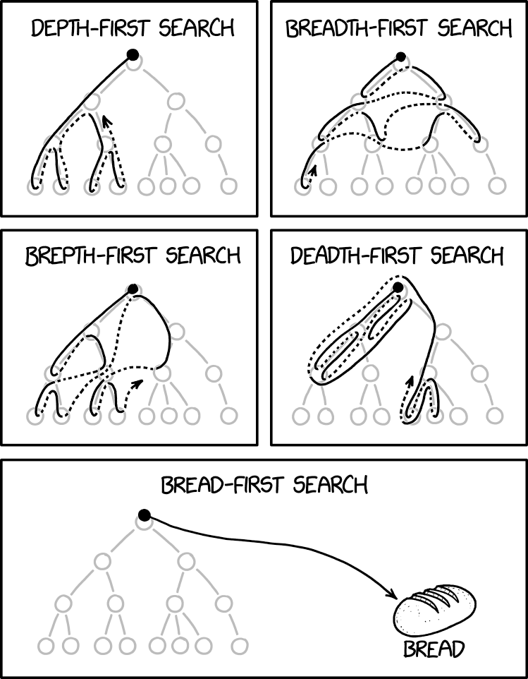
Traverse graph starting from a given vertex, processing vertices in the order they can be reached. Only visit each vertex once, keeping track of the set of already visited vertices. Often implemented using a FIFO queue.

The traversal can be visualized as a tree, where we visit nodes in top-down, left-right order.

BFS(v):
    Initialize a FIFO queue with a single item v
    Initialize a set of seen vertices with a single item v
    while the queue is not empty:
        u = pop the next element in the queue
        Visit vertex u
        for each edge (u, w):
            if w is not already seen:
                add it to the queue
                add it to set of seen vertices

Note

When we first add a vertex to the queue, we mark it as seen, so it can’t be added to the queue again. Since there are only finitely-many vertices, BFS will eventually terminate.

Each edge gets checked at most once (in each direction), so if there are n vertices and m edges, the runtime is \(\Theta(n+m)\) (assuming you can get the edges out from a vertices in constant time).

DFS

Traverse like BFS, except recursively visit all descendants of a vertex before moving on to the next one (at the same depth). This can be implemented without a queue, only using the call stack.

DFS(v):
    mark v as visited
    for each edge (v, u):
        if u is not visited, DFS(u)

Note

As with DFS, we visit each vertex at most once, and process each edge at most once in each direction, so runtime is \(\Theta(n+m)\).

We call \(\Theta(n+m)\) linear time for graphs with n vertices and m edges.

Representing Graphs

• Adjacency lists: for each vertex, have a list of outgoing edges

  • Allows for linear iteration over all edges from a vertex

  • Checking if a particular edge exists is expensive

  • Size for n vertices, m edges = \(\Theta(n + m)\)

• Adjancency matrix: a matrix with entry \((i, j)\) indicating an edge from i to j

  • Constant time to check if a particular edge exists

  • but the size based on number of vertices is \(\Theta(n^2)\)

A graph with n vertices has \(\leq {n \choose 2}\) edges if undirected, or \(\leq n^2\) if directed and we allow self-loops (or \(\leq n(n-1)\) if no self loops).

In all cases, \(m=O(n^2)\). This makes the size of an adjacency list \(O(n^2)\).

If we really have a ton of edges, the two representations are the same; but if you have a sparse graph (\(m << n^2\)), then the adjacency list is more memory-efficient.

This means that a \(\Theta(n^2)\) algorithm can run in linear time (\(\Theta(n+m)\)) on dense graphs because \(m = \Theta(n^2)\).

So \(\Theta(n^2)\) is optimal for dense graphs, but not for sparse graphs.

More Problems

Cyclic Test

testing if a graph is cyclic

• use DFS to traverse, keep track of vertices visited along the way

• if we find an edge back to any such vertex, we have a cycle

Topological Order

• Finding a topological ordering of a DAG (directed acyclic graph)

  • an ordering \(v_1, v_2, v_n\) of the vertices such that if \((v_i, v_j) \in E\), then \(i < j\)

  • we can find topological order using postorder traversal in DFS

    • after DFS has visited all descendants of a vertex, prepend the vertex to the topological order

  • make sure to iterate all connected components of the graph, not just one

def Topo-Sort(G):
    for v in V:
        if v is not visited:
            Visit(v)

def Visit(v):
    mark v as visited
    mark v as in progress // temporarily
    for edges (v, u) in E:
        if u is in progress, G is cyclic // there is no topological order
        if u is not visited:
            Visit(u)
    mark v as not in progress
    prepend v to the topological order

Minimum Spanning Tree

Suppose you need to wire all houses in a town together (represented as a graph, and the edges represent where power lines can be built), Build a power line to use the minimal amount of wire.

Given a weighted graph, (i.e. each edge has a numerical weight), we want to find a minimum spanning tree: a selection of edges of G that connects every vertex, is a tree (any cycles are unnecessary), and has least total weight.

Kruskal’s Algorithm

Main idea: add edges to the tree 1 at a time, in order from least weight to largest weight, skipping edges that would create a cycle

This is an example of a greedy algorithm, since it picks the best available option at each step.

We use a disjoint-set forest to keep track of sets of connected components.

Initially, all vertices are in their own sets. When we add an edge, we Union the sets of its two vertices together. If we would add an edge that would connect two vertices in the same set, we skip it (it would cause a cycle).

def Kruskal(G, weights w):
    initialize a disjoint-set forest on V
    sort E in order of increasing w(e)
    while all vertices are not connected:  // i.e. until n-1 edges are added
        take the next edge from E, (u, v)
        if Find(u) != Find(v):
            add (u, v) to the tree
            Union(u, v)

Runtime:

• L2: \(\Theta(n)\)

• L3: \(\Theta(m \log m)\)

• L4: \(m\) iterations of the loop worst case

  • Note that this lets us use the amortized runtime of Find and Union

  • L6: two finds (\(\Theta(\alpha(n))\) each)

  • L8: and a union (\(\Theta(\alpha(n))\))

• Note that \(m \alpha(n) < m \log m\) since \(n \leq m\)

So the total runtime is \(\Theta(m \log m) = \Theta(m \log n)\) (since \(m = \Omega(n)\) since G is connected).

This assumes G is represented by an adjacency list, so that we can construct the list E in \(\Theta(m)\) time.

Prim’s Algorithm

Main idea: build the tree one vertex at a time, always picking the cheapest vertex

Need to maintain a set of vertices S which have already been connected to the root; also need to maintain the cost of all vertices which could be added next (the “frontier”).

Use a priority queue to store these costs: the key of vertex \(v \notin S\) will be \(\min w((u, v) \in E), u \in S\)

After selecting a vertex v of least cost and adding it to S, some vertices may now be reachable via cheaper edges, so we need to decrease their keys in the queue.

def Prim(G, weights w, root r):
    initialize a PQ Q with items V  // all keys are infinity except r = 0
    initialize an array T[v] to None for all vertices v in V
    while Q is not empty:
        v = Delete-Min(Q)  // assume delete returns the deleted elem
        for each edge (v, u):
            if u is in Q and w(v, u) < Key(u):
                Decrease-Key(Q, u, w(v, u))
                T[u] = (v, u)  // keep track of the edge used to reach u
    return T

Runtime:

• n iterations of the main loop (1 per vertex), with 1 Delete-Min per iteration

• every edge considered at most once in each direction, so at most m Decrease-Key

• we use a Fibonacci heap, (Delete-Min = \(\Theta(\log n)\), Decrease-Key = \(\Theta(1)\) amortized)

• so the total runtime is \(\Theta(m + n \log n)\).

Note

We can compare the runtime of these two algorithms on sparse and dense graphs:

On a sparse graph, i.e. \(m = \Theta(n)\), the two have the same runtime: \(\Theta(n \log n)\).

On a dense graph, i.e. \(m = \Theta(n^2)\), Kruskal’s ends up with \(\Theta(n^2 \log n)\) and Prim’s with \(\Theta(n^2)\).

Proofs

Need to prove that the greedy choices (picking the cheapest edge at each step) leads to an overall optimal tree.

Key technique: loop invariants: A property P that:

1. is true at the beginning of the loop

2. is preserved by one iteration of the loop (i.e. if P is true at the start of the loop, it is true at the end)

By induction on the number of iterations, a loop invariant will be true when the loop terminates. For our MST algorithms, our invariant will be: The set of edges added to the tree so far is a subset of some MST.

If we can show that this is an invariant, then since the tree we finally return connects all vertices, it must be a MST.

Lemma (cut property): Let \(G=(V,E)\) be a connected undirected graph where all edges have distinct weights. For any \(S\subseteq V\), if \(e \in E\) is the cheapest edge from \(S\) to \(V-S\), every MST of \(G\) contains \(e\).

Kruskal’s

Thm: Kruskal’s alg is correct.

Pf: We’ll establish the loop invariant above.

Base case: before adding any edges, the edges added so far is \(\emptyset\), which is a subset of some MST.

Inductive case: suppose the edges added so far are contained in an MST \(T\), and we’re about to add the edge \((u, v)\).

• Let \(S\) be all vertices already connected to \(u\).

• Since Kruskal’s doesn’t add edges between already connected vertices, \(v \notin S\)

• Then \((u, v)\) must be the cheapest edge from \(S\) to \(V-S\), since otherwise a cheaper edge would have been added earlier in the algorithm, and then \(v \in S\)

• Then by the cut property, every MST of \(G\) contains \((u, v)\)

• In particular, \(T\) contains \((u, v)\), so the set of edges added up to and including \((u, v)\) is also contained in \(T\), which is a MST

• So the loop invariant is actually an invariant, and by induction it holds at the end of the algorithm

So all edges added are in an MST, and since they are a spanning tree, they are a MST. Since the algorithm doesn’t terminate until we have a spanning tree, the returned tree must be a MST.

Prim’s

Idea: Let \(S\) be the set of all vertices connected so far. Prim’s then adds the cheapest edge from \(S\) to \(V - S\).

So by the cut property, the newly added edge is part of every MST. The proof follows as above.

Cut Property

Proof of the following lemma, restated from above:

Let \(G=(V,E)\) be a connected undirected graph where all edges have distinct weights. For any \(S\subseteq V\), if \(e \in E\) is the cheapest edge from \(S\) to \(V-S\), every MST of \(G\) contains \(e\).

Suppose there was some MST \(T\) which doesn’t contain \(e=(u, v)\). Since \(T\) is a spanning tree, it contains a path \(P = (u, ..., v)\). Since \(u \in S\) and \(v \notin S\), \(P\) contains some edge \(e' = (u', v')\) with \(u' \in S, v' \notin S\). We claim that exchanging \(e\) for \(e'\) will give a spanning tree \(T'\) of lower weight than \(T\), which contradicts \(T\) being an MST.

First, \(T'\) has smaller weight than \(T\), since \(e\) is cheaper than \(e'\) by definition.

Next, \(T'\) connects all vertices, since \(T\) does, and any path that went through \(e'\) can be rerouted to use \(e\) instead: follow \(P\) backwards from \(u'\) to \(u\), take \(e\) from:math:u to \(v\), then follow \(P\) backwards from \(v\) to \(v'\), and then continue the old path normally. (e.g. \((a, ..., u', v', ..., b) \to (a, ..., u', ..., u, v, ..., v', ..., b)\))

Finally, \(T'\) is also acyclic, since adding \(e\) to \(T\) produces a single cycle, which is then broken by removing \(e'\).

So \(T'\) is a spanning tree of lower weight than \(T\) - contradiction! Therefore every MST of G must contain the edge e.

Note

To relax the assumption of distinct edge weights, imagine adding tiny extra weights to break any ties in the MST algorithm; if the changes in the weights are sufficiently small, then any MST of the new graph is also an MST of the original (see hw4).

Single-Source Shortest Paths

Given a directed graph with nonnegative edge weights (lengths) and a start vertex \(s\), find the shortest paths from \(s\) to every other vertex (shortest = minimum total length/weight). (Assume every vertex is reachable from s.)

To represent the shortest paths, we use a shortest-path tree: each vertex stores the edge that should be used to reach it from s along the shortest path.

Ex. For this graph, starting from vertex z, the shortest-path tree T is:

T[x] = (z, x)
T[y] = (w, y)
T[w] = (z, w)

Dijkstra’s Algorithm

Greedy algorithm for building the shortest-path tree. Very similar to Prim’s, but the cost of a vertex is the length of the shortest known path to reach it from s

Idea: Maintain a set of vertices S already added to the shortest-path tree; for these vertices, we know their distance d(v) from s. At each step, add a vertex \(v \notin S\) which minimizes \(d(u) + w(u, v)\) over all \(u \in S\) with \((u, v) \in E\)

def Dijkstra(G, weights w, source s in V):
    Initialize a PQ Q with items V; all keys d(v) = inf except d(s) = 0
    Initialize an array T[v] to None for all v in V
    while Q is not empty:
        u = Delete-Min(Q)
        for each edge (u, v) in E:
            if v in Q and d(v) > d(u) + w(u, v):
                Decrease-Key(Q, v, d(u) + w(u, v))
                T[v] = u
    return T

Runtime: Same as Prim’s algorithm - \(\Theta(m + n \log n)\) using a Fibonacci heap

Proof

To prove correctness, we’ll use the following loop invariant I:

for all vertices v popped off the queue so far:

• \(d(v)\) is the distance from s to v and

• there is a path \(P_v\) from s to v in T which is a shortest path

  • \(P_v=(v, T[v], T[T[v]], ..., s)\) reversed

To show I is an invariant, need to prove it is true initially and it preserved by one iteration. If S is the set of popped-off vertices, then initially \(S = \emptyset\) so I holds vacuously.

Suppose I holds at the beginning of an iteration. If we pop vertex v, and \(T[v]=(u, v)\), then \(u \in S\), so \(P_u\) is a shortest path from s to u and \(d(u)\) is the distance from s to u. Also \(d(v) = d(u) + w(u, v)\) by line 8, which is the length of the path \(P_v\).

Now suppose there were a shorter path P from s to v. Since \(v \notin S\), P must leave S at some point: let the first edge leaving S be \((x, y)\). Since \(x \in S\), we previously considered the edge \((x, y)\) and therefore \(d(y) \leq d(x) + w(x, y)\). Also, since \(y \notin S\), the algorithm selected v to pop before y, so \(d(v) \leq d(y)\). Then \(d(v) \leq d(x) + w(x, y)\) but the length of P is \(d(x) + w(x, y)\), and \(P_v\) has length \(d(v)\), so P cannot be shorter than \(P_v\). This is a contradiction, so \(P_v\) is in fact a shortest path from s to v.

Then \(d(v)\) is the distance from s to v, so I holds after the end of the loop. Therefore I is an invariant, and by induction it holds when the algorithm terminates. Since all vertices are popped off when the algorithm terminates, T must then be a shortest path’s tree (and \(d(v)\) is the distance from s to v for all v)

Related Problems

Shortest-Paths in a DAG

Can do better than Dijkstra’s using a topological order on the vertices:

\(d(v)=\min_{(u, v) \in E} [d(u)+w(u, v)]\) (by convention, infinity if there are no edges (u, v))

\(d(s) = 0\)

Iteratively compute \(d(v)\) in topological order - whenever \(d(u)\) is needed, it has already been computed. This works even if there are negative weights.

Shortest-Paths With Negative Weights

Use the Bellman-Ford alg. (examined later)

All-Pairs Shortest-Paths

Find the shortest path from u to v for any pair of vertices (u, v)

Could run Dijkstra from every start vertex; for dense graphs use the Flord-Warshall alg.

Greedy Algorithms

Idea: build up a solution incrementally, taking the best available option at each step (e.g. Kruskal/Prim)

This kind of “local” reasoning doesn’t necessarily yield a globally optimal solution. The trick in designing a greedy algorithm is to find a greedy strategy that you can prove gives a global optimum.

Interval Scheduling Problem

Have a resource which can only be used by one person at a time, and people want to use it at different time periods.

We have n requests of the form \((s(i), f(i))\) giving the starting and finishing times. Want to find the largest possible subset (by cardinality) of non-overlapping (compatible) requests.

Natural greedy approach:

1. Use some heuristic to select a request i and add it to our set

2. Delete all requests incompatible with i

3. Repeat until there are no requests left

Possible heuristics:

• Earliest request (does not work)

• Shortest request (does not work)

• Fewest conflicts (does not work)

• Request finishing first (works!)

  • Intuition: maximize the time remaining in which to service other requests

Optimality

How do you prove optimality of a greedy strategy?

Exchange Argument

Take an optimal solution and transform it into the solution that the algorithm outputs without increasing its cost.

e.g. proof of cut property: we took an MST and showed that using the edge chosen by Kruskal/Prim would decrease its cost

Inductive Argument

Break up an optimal solution into stages, and show inductively that the greedy algorithm does at least as well as the optimal solution in each successive stage

ISP

We use the inductive argument to prove the optimality of the “smallest finishing time” heuristic for the interval scheduling problem:

Call the set of intervals chosen by the algorithm A.

First, A is compatible, since we throw out incompatible requests each time we add a new request to A.

Take an optimal set of requests O. Need to show that \(|A| = |O|\).

Let \(i_1, i_2, ..., i_k\) be the intervals of A in the order they were added.

Let \(j_1, j_2, ..., j_m\) be the intervals of O in left-to-right order.

Then need to show that \(k=m\). Intuition for our heuristic was to make the resource available as soon as possible, so let’s prove that (i.e., for all \(r \leq k, f(i_r) \leq f(j_r)\)). Prove by induction on r.

Base Case: \(r=1\) - Algorithm picks \(i_1\) to be the request with smallest finishing time, so \(f(i_1)\leq f(j_1)\).

Inductive Case: \(r > 1\) - Assume that \(f(i_{r-1}) \leq f(j_{r-1})\). Since \(j_{r-1}\) is compatible with \(j_r\), \(f(j_{r-1}) \leq s(j_r)\).

So by the hypothesis, \(f(i_{r-1}) \leq f(j_{r-1}) \leq s(j_r)\), so \(i_{r-1}\) is compatible with \(j_r\), and therefore \(j_r\) is one of the options considered when picking \(i_r\).

Since the algorithm picks the request with least finishing time amongst those consistent with the previously-chosen requests, \(f(i_r) \leq f(j_r)\).

So by induction, \(f(i_r) \leq f(j_r) \forall r \leq k\).

Now suppose that A was not optimal, i.e. \(k < m\). By above, \(f(i_k) \leq f(j_k)\). Since O is compatible, \(f(j_k) \leq s(j_{k+1})\), so \(j_{k+1}\) is compatible with \(i_k\), and the algorithm should not have terminated after \(i_k\) - contradiction.

Scheduling to Minimize Lateness

Have n jobs which have durations \(t_i\) and deadlines \(d_i\). If we start job i at time \(s(i)\) and finish it at \(f(i) = s(i) + t_i\), the lateness \(l_i = \max(0, f(i)-d_i)\).

We want a schedule minimizing the maximum lateness \(\max_i l_i\).

A greedy strategy which is optimal: “earliest deadline first”: sort jobs in order of increasing \(d_i\) and execute them in that order.

We use the exchange argument to prove optimality: convert an optimal schedule into the EDF schedule without increasing the maximum lateness.

Note

The EDF schedule has no gaps (idle time) between jobs.

Lemma: There is an optimal schedule with no idle time.

Note

Our EDF schedule also has no inversions: executing job i before j when \(d_i>d_j\).

Lemma: The EDF schedule is the unique idle-free schedule with no inversions, up to rearranging jobs with the same deadline (and note that such rearranging does not change the maximum lateness).

Now the idea is to take an idle-free optimal schedule, and eliminate inversions without increasing max lateness - this will then show EDF is just as good, by above lemma.

Note

Lemma: If an idle-free schedule has an inversion, it has an inversion of adjacent jobs.

Proof: Assume not. Let \((i, j)\) be a closest inversion, and let k be the job after i.

If \(d_i > d_k\), then \((i, k)\) is an adjacent inversion. (done)

Otherwise, \(d_i \leq d_k\), so \(d_k > d_j\), so \((k, j)\) is an inversion. This contradicts \((i, j)\) being a closest inversion.

Note

Lemma: Swapping the jobs of an adjacent inversion reduces the number of inversions by 1, and does not increase the maximum lateness.

Proof: Swapping i and j doesn’t change the lateness of any jobs other than i and j. Job j can only get a reduced lateness since it now ends earlier. If job i is late,

\[\begin{split}l_i & = f(i) - d_i \\ & = f(j)_{old}-d_i \\ & \leq f(j)_{old} - d_j \\ & \leq l_{j, old}\end{split}\]

So the old maximum lateness ≥ the new maximum lateness.

Thm: The EDF schedule is optimal.

Proof: Let \(S\) be an optimal idle-free schedule with fewest inversions.

If it has no inversions, its maximum lateness = that of the EDF schedule.

Otherwise, we can exchange the jobs in an adjacent inversion to get a schedule with fewer inversions, but as good maximum lateness. This contradicts the idea that S has fewest inversions.

Huffman Coding

If you want to compress data, you take advantage of the data not being completely random.

Note

Ex: Suppose you want to send a message using only letters A, B, C, D. In general, would take 2 bits per letter (e.g. A = 00. B = 01, C = 10, D = 11).

If some letters are more likely than others, could give those shorter codewords. E.g. A = 0, B = 10, C = 111, D = 100. E.g. CAAB = 1110010 = 7 bits

To be able to uniquely decode, need a prefix-free code: no codeword is a prefix of another.

Huffman coding gives an optimal prefix-free code (i.e. minimizes the expected length of the message).

Greedy algorithm to build encoding/decoding tree: repeatedly merge the nodes with least probability

Dynamic Programming

Fundamental idea: write the optimal solution to a problem in terms of optimal solutions to smaller subproblems.

When this is possible, the problem is said to have optimal substructure)

When you can do this, you get a recursive algorithm as in divide/conquer. The difference is that usually the subproblems overlap.

Weighted Interval Solving Problem

Like ISP from earlier, we have n requests for a resource with starting and finishing times, but now each request has a value \(v_i\). We want to maximize the total value of granted requests.

Goal: Find a subset S of requests which is compatible and maximixes \(\sum_{i \in S} v_i\).

Let’s sort the requests by finishing time, so request 1 finishes first, etc.

To use dynamic programming, we need to write an optimal solution in terms of optimal solutions of subproblems. Note that an optimal solution O either includes the last request n or doesn’t.

If \(n \in O\), then O doesn’t contain any intervals overlapping with n; let \(p(n)\) be the last interval in the order that doesn’t overlap with n.

Then intervals \(p(n)+1, p(n)+2, ..., n-1\) are excluded from O, but O must contain an optimal solution for intervals \(1, 2, ..., p(n)\).

Note

If there were a better solution for intervals \(1, 2, ..., p(n)\), then we could improve O without introducing any conflicts with n (exchange argument).

If instead \(n\notin O\), then O must be an optimal solution for intervals \(1, 2, ..., n-1\).

Note

If O was not an optimal solution for intervals \(1, 2, ..., n-1\), we could improve O as above.

So, either O is an optimal solution for intervals \(1, ..., p(n)\) plus n, or it is an optimal solution for intervals \(1, ..., n-1\).

If we then let \(M(i)\) be the maximal total value for intervals [1, i], we have:

\[\begin{split}M(i) & = \max(M(p(i)) + v_i, M(i-1)) \text{ for } i > 1 \\ M(1) & = v_1\end{split}\]

This recursive equation gives us a recursive algorithm to compute the largest possible total value overall, which is \(M(n)\). We can then read off which intervals to use for an optimal set:

• if \(M(n) = M(p(n)) + v_n\), then include interval n

• if \(M(n) = M(n-1)\), then exclude interval n

then continue recursively from \(p(n)\) or \(n-1\) respectively.

Runtime

Recursion tree has 2 subproblems, but depth \(\approx n\). So in total, the runtime is \(\approx 2^n\).

But there are only n distinct subproblems: \(M(1), M(2), ..., M(n)\). Our exponentially many calls are just doing the same work over and over again.

Solution: memoization - whenever we solve a subproblem, save its solution in a table; when we need it later, just look it up instead of doing further recursion.

Here, we use a table \(M[1..n]\). Each value is then computed at most once, and work to compute a value is constant, so total runtime will be linear (assuming \(p(i)\) is computed).

Another way to think about memoization: it turns a recursion tree into a DAG by collapsing identical nodes together.

Note

Instead of memoization on a recursive algorithm, we can also eliminate recursion and just compute the “memo table” iteratively in a suitable order.

In the example above, could just compute M[1], M[2], …, M[n] in increasing order: then all subproblems needed to compute M[i] will already have been computed (since M[i] only depends on M[j] with j<i)

M[1] = v1
for i from 2 to n:
    M[i] = max(M[p(i)] + vi, M[i - 1])

TLDR: Dynamic programming = recursive decomposition into subproblems + memoization

Design

Main steps for designing a dynamic programming algorithm:

1. Define a notion of subproblem; there should only be polynomially-many distinct subproblems

2. Derive a recursive equation expressing the optimal solution of a subproblem in terms of optimal solutions to “smaller” subproblems

3. Express the solution to the original problem in terms of one or more subproblems

4. Work out how to process subproblems “in order” to get an iterative algorithm

Edit Distance

Levenshtein Distance

Distance metric between strings, e.g. “kitten” and “site”.

\(d(s, t)\) = minimum number of character insertions, deletions, or substitutions (replacing a single character with another) needed to turn s into t.

Ex:

kitten
sitten
siten
site

This is the shortest sequence of transformations, so \(d(kitten, site) = 3\). Very useful for approximate string matching, e.g. spell checking, OCR, DNA sequence alignment (see textbook)

Naive algorithm (checking all strings reachable with 1 op, 2 ops, etc) could take exponential time - let’s improve with dynamic programming.

Problem

Given strings s[1..n] and t[1..m], compute \(d(s, t)\). To divide into subproblems, let’s look at prefixes of s and t.

Let \(D(i, j)\) be the edit distance between s[1..i] and t[1..j]. We ultimately want to compute \(D(n, m)\).

Let’s find a recursive equation for \(D(i, j)\). Suppose we had an optimal sequence of operations transforming s[1..i] into t[1..j]. Without loss of generality, we can assume the operations proceed from left to right; then can view the sequence as an “edit transcript” saying for each character of s what operation(s) to perform, if any.

Ex: (S = sub, I = insert, D = delete, M = noop)

kitten -(sub k)> sitten -(del t)> siten -(del n)> site

transcript: SMMDMD

Solution

Look at the last operation in the transcript. Several possibilities:

• If I, the sequence is an optimal seq. turning s[1..i] into t[1..j-1] followed by the insertion of t[j], so \(D(i, j) = D(i, j-1)+1\).

• If D, the seq. is an optimal one turning s[1..i-1] into t[1..j], followed by deleting s[i], so \(D(i, j) = D(i-1, j) + 1\).

• If S, the seq. is an optimal one turning s[1..i-1] into t[1..j-1], followed by turning s[i] into t[j], so \(D(i, j) = D(i-1, j-1) + 1\).

• If M, the seq. is an optimal one turning s[1..i-1] into t[1..j-1], so \(D(i, j) = D(i-1, j-1)\).

The optimal sequence will take whichever option yields the smallest value of D, so we have

\[\begin{split}D(i, j) & = \min(D(i, j-1)+1, D(i-1, j)+1, D(i-1, j-1)+c) \\ & \text{where } c = 0 \text{ if s[i] = t[j] or } 1 \text{ otherwise} \\ D(0, j) & = j \\ D(i, 0) & = i\end{split}\]

Note

For the base cases, we can use a sequence of insertions/deletions to get from an empty string to another (or vice versa).

Runtime

How long does the recursive algorithm with memoization take to compute \(D(n, m)\)?

• Total number of distinct subproblems: \(\Theta(nm)\)

• Time for each subproblem: \(\Theta(1)\) (only look at a constant number of previously computed values)

So the total runtime is \(\Theta(nm)\).

Note

The memo table takes \(\Theta(nm)\) memory, but recursion only depends on current and previous value of j, so it is enough to save only the current and previous row of the table.

This reduces the memory needed to \(\Theta(m)\).

Bellman-Ford Algorithm

single-source shortest paths with negative weights

Note

If there is a cycle with negative weight (a “negative cycle”), no shortest path may exist.

The BF algorithm can detect this.

Idea

Compute distance \(d(v)\) to each vertex v from source s by dynamic programming.

Note that this is similar to the shortest-path algorithm for DAGs. However, a naive attempt won’t work since the graph can have cycles, which would lead to infinite recursion when trying to compute \(d(v)\).

To fix this problem, we introduce an auxiliary variable in our definition of the subproblems. Here, given source vertex s, let \(D(v, i)\) be the length of the shortest path from s to v using at most i edges. This prevents infinite recursion since we’ll express \(D(v, i)\) in terms of D for smaller values of i.

Solution

Lemma: If there are no negative cycles, the shortest path from s to v passes through each vertex at most once, so \(d(v) = D(v, n-1)\).

To get a recursion for \(D(v, i)\), consider a shortest path from s to v using at most i edges: either it has exactly i edges, or \(\leq i-1\) edges.

• If \(\leq i-1\) edges, then \(D(v, i) = D(v, i-1)\)

• If exactly i edges, call the last edge \((u, v)\); then we have \(D(v, i) = D(u, i-1) + w(u, v)\).

So, minimizing over all possible cases (including the choice of u):

\[\begin{split}D(v, i) & = \min(D(v, i-1), \min_{(u, v) \in E} (D(u, i-1) + w(u, v))) \\ D(v, 0) & = \begin{cases} 0 & v = s \\ \infty & \text{ otherwise} \end{cases}\end{split}\]

Now we can compute \(D(t, n-1)\) to get the distance \(d(t)\) using this formula using memoization as usual.

Runtime

Total number of distinct subproblems: n choices for v and n choices for i = \(\Theta(n^2)\)

Notice for each subproblem, we iterate over all incoming edges to v. So for each i, only need to consider each edge exactly once.

Therefore, the total runtime is \(\Theta(nm)\).

Network Flow

Idea: model a network as a graph where some material (water, data, etc) flows along edges, but each edge has a maximum capacity for flow.

Like MST and shortest paths, many problems from many areas (e.g. transportation, communication, image processing) can be put in this form.

Flow Networks

A flow network is a directed graph \(G=(V,E)\) where each edge e has a nonnegative capacity \(c_e\) (for simplicity, assume capacities are integers).

There are also designated source and sink nodes \(s, t \in V\).

All other nodes are called internal nodes.

We assume every node has at least 1 edge connected to it (otherwise we remove it).

S-T Flow

An s-t flow (or simply “flow”) is a function \(f: E \to \mathbb{R}\) (where \(f(e)\) is the amount of flow along edge e) satisfying:

1. For all \(e \in E, 0 \leq f(e) \leq c_e\) (flow does not exceed capacity

2. For all internal nodes v, \(\sum_{(u, v)\in E} f(e)= \sum_{(v, u)\in E} f(e)\) (flow into v = flow out of v; conservation of mass)

Flow into u: \(f(s, u) = 20\)

Flow out of u: \(f(u, v) + f(u, t) = 10 + 10 = 20\)

The value of a flow f is the total flow coming out of the source: \(v(f) = \sum_{(s, u) \in E} f(e)\).

In the example above, \(v(f) = f(s, u) + f(s, v) = 20 + 0 + 20\).

Maximum-Flow Problem

Given a flow network, find a flow with the largest possible value.

To solve this, there’s a natural greedy approach: given a flow, incrementally try to increase the flow along some path from s to t.

1. Start with 0 flow at each edge: this is a valid flow.

2. Given a path from s to t, look at the minimum capacity of edges along it: this is the bottleneck for adding flow along the path. Add this much flow along each edge.

Ex: Consider the path \((s, u, v, t)\). Minimum capacity is 20, so we could “push” 20 units of flow along the path to get a flow of higher value.

We could then try to push more flow along a different path, etc. However, in this example, we get stuck! There are no more paths we can push flow on, but this flow is not optimal.

In order to get an optimal flow (of value 30 in this example), we would need to decrease the flow from u to v from 20 to only 10. To keep track of which edges can be increased or decreased, we use the residual graph.

The residual graph \(G_f\) of a flow f has the same vertices as G, and for every edge \(e = (u, v)\) of G:

1. If \(f(e) < c_e\), there is \(c_e - f(e)\) residual capacity (unused capacity), so we add a forward edge \((u, v)\) to \(G_f\) with capacity \(c_e - f(e)\).

2. If \(f(e) > 0\), we could decrease the flow by up to \(f(e)\), so we add a backward edge \((v, u)\) to \(G_f\) with capacity \(f(e)\).

Ex: In the flow above, \(G_f\) is:

Note

For each edge of G, there can be 1 or 2 edges in \(G_f\).

We’ll call a path from s to t in \(G_f\) which doesn’t repeat vertices an augmenting path. Given such a path, we can augment the flow f as follows: if b is the weight of the least-weight edge along the path, then we consider each edge of the path in turn:

• if it is a forward edge, increase the flow along it in G by b

• if it is a backward edge, decrease the flow along the reverse edge in G by b.

Lemma: The result of augmenting a flow along any augmenting path is a valid flow of higher value.

This then enables a greedy approach to max flow:

Ford-Fulkerson Method

• start with the all-zero flow f

• while there is a path from s to t in \(G_f\):

  • take any augmenting path p

  • augment f along p

• return f

Termination and Runtime

Invariant: Flow along each edge is an integer.

• True initially, since we start with the all-zero flow

• If true at one iteration, the residual capacities are all integers since the flows and capacities are integers. So the bottleneck b is an integer, and the new flow will all be integers.

So the value of the flow increases every iteration (see lemma) and is an integer, and since it can’t exceed \(\sum_{e=(s,v)\in E}c_e\), the value of the flow has to eventually stop growing so the loop must eventually terminate.

If the value of the maximum flow is F, there are in fact at most F iterations, since \(b \geq 1\). So if the network has n vertices and m edges, we can implement FF in \(O(mF)\) time:

1. Building the residual graph takes \(O(n+m)\) time, which is \(O(m)\) since each vertex has at least one edge

2. Finding an augmenting path with BFS/DFS takes \(O(m)\) time

3. Augmenting the flow requires iterating over the path and takes \(O(m)\)

Optimality

Idea: Flow from s to t cannot exceed the total capacity of edges crossing a cut which separates s from t.

A partition of V into two sets \((A, B)\) with \(s\in A, t\in B\) is an s-t cut.

The capacity of the cut is the total capacity of all edges from A to B:

\[\begin{split}c(A,B) & =\sum_{e=(u, v)\in E, u \in A, v \in B}c_e \\ & = \sum_{e \text{ out of } A}c_e\end{split}\]

Given a flow f, let \(f^{out}(A) = \sum_{e \text{ out of } A} f(e)\) and \(f^{in}(A) = \sum_{e \text{ into } A} f(e)\)

Lemma

\(v(f)=f^{out}(A)-f^{in}(A)\)

Proof: By definition, \(v(f)=f^{out}(s)\). Also \(f^{in}(s)=0\) since s has no incoming edges. So \(v(f)=f^{out}(s)-f^{in}(s)\). Also, by conservation of flow, for any \(v \in A\) besides s, \(f^{out}(v)=f^{in}(v)\). So \(v(f)=\sum_{v\in A}(f^{out}(v)-f^{in}(v))\). Now consider the contribution of every edge \(e=(u, v)\) to this sum:

• If an edge from A to A, its flow \(f(e)\) appears as a positive term in \(f^{out}(u)\) and a negative term in \(f^{in}(v)\), which cancel out.

• If an edge from A to B, it contributes \(f(e)\) to the sum

• If an edge from B to A, it contributes \(-f(e)\)

• If an edge from B to B, it contributes 0

So the sum is equivalent to

\[\begin{split}& \sum_{e \text{ out of } A} f(e) - \sum_{e \text{ into } A} f(e) \\ & = f^{out}(A)-f^{in}(A).\end{split}\]

Corollary: For any flow f and s-t cut \((A, B), v(f)\leq c(A, B)\).

Theorem

When FF algorithm returns f, there is an s-t cut \((A, B)\) such that \(v(f)=c(A,B)\).

Proof: When FF terminates, there is no path from s to t in \(G_f\). So if A is all vertices reachable from s in \(G_f\), and B is all other vertices, \((A, B)\) is an s-t cut.

There are no edges from A to B in \(G_f\), since otherwise the destination in B would be reachable from s.

So for any edge e from A to B in the original graph G, we must have \(f(e)=c_e\), since otherwise there would be a forward edge from A to B in \(G_f\).

Likewise, for any edge e from B to A in G, we must have \(f(e)=0\), since otherwise there would be a backward edge from A to B in \(G_f\).

Now by earlier lemma:

\[\begin{split}v(f) & = f^{out}(A) - f^{in}(A) \\ & = \sum_{e \text{ out of } A} f(e) - \sum_{e \text{ into } A} f(e) \\ & = \sum_{e \text{ out of } A} c_e \\ & = c(A, B).\end{split}\]

Corollary: Since no flow has value greater than the capacity of a cut, the flow returned by FF is optimal.

Corollary: The cut \((A, B)\) from the theorem above is a minimum cut: its capacity is as small as possible. (If there were one with a smaller capacity, the flow would have to have a smaller value)

This means we can use FF to find a minimum s-t cut in a graph: run it to find the flow f, then build \((A, B)\) as in the theorem.

Theorem (Max-Flow Min-Cut): In any flow network, the maximum value of an s-t flow is the minimum value of an s-t cut.

Note

Since FF always finds a flow with integer flows on all edges, there is always a maximum flow of this form.

Runtime Revisited

Our runtime bound of \(O(mF)\) with F being the value of the max-flow isn’t good when the capacities in the network are large (F could be large). But it turns out that if you use BFS to find the shortest augmenting path, the algorithm takes at most \(O(nm^2)\) time.

This choice of path is called the Edmonds-Karp algorithm.

Applications

• Routing problems (get data from point A to B, maximizing throughput)

• Matching problems, e.g. bipartite matching

Bipartite Matching

Suppose we have n workers with different skills, and various jobs to do which some subsets of the workers are qualified to do. We want to assign workers to jobs so that as many jobs get done as possible, with no worker assigned multiple jobs and no job assigned multiple workers.

Model this problem using a bipartite graph: vertices for workers and jobs, with edges indicating who can do which jobs.

Then we want to find a maximum matching: a set of edges M where no two edges share a vertex and is as large as possible.

Idea: construct a network for instance such that the maximum flow is obtained by matching as many workers to jobs as possible.

Think of each worker as having 1 unit of work, which can be allocated to any of the jobs they can perform.

• Add source node s and capacity 1 edges to each worker

• Add capacity 1 edges from each worker to each possible job they can do

• Add capacity 1 edges from each job to a sink node t

To show this works, need to prove 2 directions:

• If there is a matching with k edges, there is a flow of value k: flow 1 unit to each of the k workers assigned a job, then along the matched edges to their corresponding jobs, then to t.

• Conversely, given a maximum flow with value k from FF, we can assume all flows on all edges are integers. Then there must be k jobs with 1 unit of flow coming out, and the rest have 0.

  • For those k jobs, they must have 1 unit of flow coming from a unique worker.

  • We can assign that worker to this job and get a valid assignment.

So every maximum matching corresponds to a maximum flow, and vice versa, and we can use FF to find such max a flow, and reconstruct the matching.

Since the maximum flow value is at most n (all workers assigned to jobs), the runtime of FF will be \(O(nm)\).

Image Segmentation

Suppose we want to identify which parts of an image are foreground/background, e.g. separating people from scenery.

Two types of criteria for deciding if a pixel is a part of the foreground:

1. A pixel may be more likely to be foreground due to color, position in image, etc. Say we have nonnegative likelihoods \(a_i\) and \(b_i\) for pixel i being foreground/background.

2. A pixel which is adjacent to other foreground pixels is likely in the foreground. For each pair \((i, j)\) of adjacent pixels, say we have a penalty \(p_{ij} \geq 0\) for putting one in the foreground but not the other.

The best segmentation is then a partition of the pixels \((A, B)\) maximizing

\[\begin{split}q(A, B) = \sum_{i\in A} a_i + \sum_{j \in B} b_j - \sum_{(i, j) \text{ adjacent} \\ \text{1 in A}} p_{ij}\end{split}\]

Solving

To find the best partition, we observe that segmentations look like cuts in a graph, since they both partition pixels/vertices into 2 disjoint groups.

Can we set up a flow network s.t. the best segmentation corresponds to a minimum cut?

Issue: need to maximize \(q\), not minimize. But notice that \(q(A, B)\) is at most \(Q=\sum_i (a_i+b_i)\). So let’s minimize:

\[\begin{split}q'(A, B) = Q-q(A,B) = \sum_{i\in A} b_i + \sum_{j \in B} a_j + \sum_{(i, j) \text{ adjacent} \\ \text{1 in A}} p_{ij}\end{split}\]

Now we need to encode \(q'(A,B)\) as the capacity of a cut in some network.

We’ll add source and sink vertices s and t, and think of an s-t cut \((A, B)\) as representing a segmentation where all pixels in A are in the foreground, and the rest are in the background. We’ll encode each item above as the capacity of an edge crossing the cut.

• Add an edge from pixel i to the sink t with capacity \(b_i\): then if \(i \in A\), since \(t\in B\), we will get a contribution of \(b_i\) to the capacity of the cut.

• Add an edge from s to j with capacity \(a_j\): then in \(j \in B\), since \(s\in A\), we will get a contribution of \(a_j\) to the capacity of the cut.

• Add edges from pixel i to adjacent pixel j and vice versa with capacity \(p_{ij}\): then if \(i \in A\) but \(j \in B\) or vice versa, we get a contribution of \(p_{ij}\).

Then the capacity of the cut \((A,B)\) equals \(q'(A,B)\), so the minimum cut in the flow network corresponds to the best segmentation. Therefore, to find \((A,B)\) we can run FF to find the maximum flow in the network and extract the corresponding minimum cut.

Beyond 102

Interactable Problems and Optimal Runtimes

How to tell whether an algorithm is as fast as possible?

We need a lower bound on how many steps any algorithm needs to solve the problem - the subject of complexity theory. There are problems for which you can prove that no poly-time algorithm exists; however, there are many open problems in complexity theory, e.g. P v. NP

Ex: Boolean Satisfiability Problem (SAT): given a Boolean formula built up from Boolean variables with AND, OR, and NOT, is it possible for the formula to evaluate to true?

• (x OR y) AND (NOT x) is satisfiable (x=false, y=true)

• x AND (NOT x) is not

This problem has lots of practical applicattions, e.g. software verification and other formal methods problems. But there’s no known poly-time algorithm! In fact, \(SAT \in NP\) since checking if a given assignment satisfies the formula is easy. Can prove that if \(SAT \in P\), then \(P=NP\).

Note

In 103, we only examine P/NP; a current area of research is fine-grained complexity, which looks at differences between \(n^2\) and \(n^3\) time. For example, there is some evidence that edit distance can’t be computed in less than \(n^{2-\epsilon}\) time.

Transcripts

Click to download.

Week 1

1/4/2021: Introduction

1/6/2021: Algorithms/RAM Model

1/8/2021: Asymptotic Notation

Week 2

1/11/2021: Examples and Recurrence

1/13/2021: Induction and Master Theorem

1/15/2021: Divide/Conquer and Mergesort

Week 3

1/20/2021: D/C Integer Multiplication

1/22/2021: D/C Closest Points

Week 4

1/25/2021: Priority Queues

1/27/2021: Amortized Runtimes (no transcript available)

1/29/2021: Graphs (no transcript available)

Week 5

2/1/2021: BFS/DFS (no transcript available)

2/3/2021: Cyclic Test/Topological Sort (no transcript available)

2/5/2021: Minimum Spanning Trees (no transcript available)

Week 6

2/8/2021: Proving Kruskal’s and Prim’s (no transcript available)

2/10/2021: Midterm

2/12/2021: Proving Cut Property, SSSP (no transcript available)

Week 7

2/17/2021: Dijkstra’s Algorithm (no transcript available)

2/19/2021: Greedy Algorithms (no transcript available)

Week 8

2/22/2021: Minimal Lateness/Huffman Coding (no transcript available)

2/24/2021: Dynamic Programming (no transcript available)

2/26/2021: Edit Distance (no transcript available)

Week 9

3/1/2021: Bellman-Ford Algorithm (no transcript available)

3/3/2021: Network Flow (no transcript available)

3/5/2021: Ford-Fulkerson Algorithm (no transcript available)

Week 10

3/8/2021: Applications of FF: Bipartite Matching

3/10/2021: Image Segmentation

Indices and tables

• Index

• Module Index

• Search Page