Algorithms
a computational procedure to solve a problem
Problem
a mapping or relation from inputs to outputs
- Input: an instance of the problem
e.g. an input might be a list of points in the convex hull problem
the encoding of the instance into a binary sequence is important - solving for lists of pairs of numbers is different than solving for strings
- Output: solution to the problem instance
e.g. a list of points making up the convex hull, in order
there can be multiple valid solutions for some problem instances, e.g. sorting
Key property of an algorithm for problem P: for any instance of P, running the algorithm on the instance will cause it to eventually terminate and return a corresponding solution
If an algorithm does so, it is called correct.
To measure the time for an algorithm to execute, we need to define “computational procedure”:
Computational Procedure
the RAM model
Idea: algorithm = program running on an abstract computer, e.g. Turing Machine (CSE 103)
The RAM model is an abstract computer that is more complex than TMs but closer to a real computer.
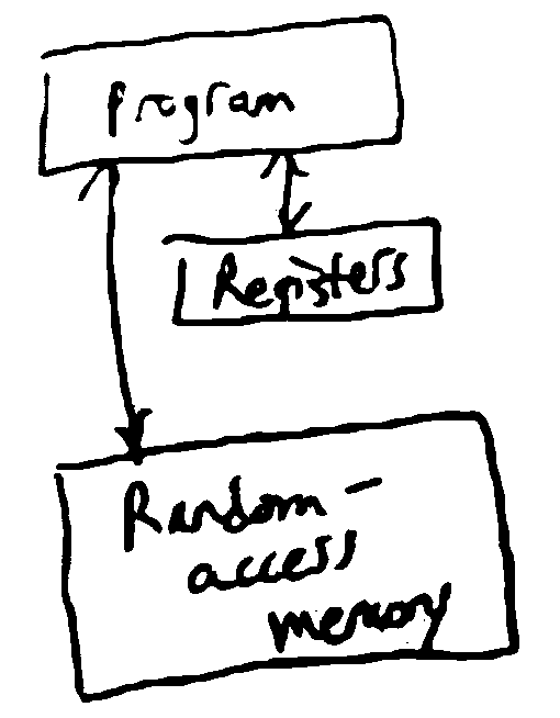
RAM Model
- registers
store some finite amount of finite-precision data (e.g. ints or floats)
- random access memory (RAM)
stores data like registers, but with infinitely many addresses
can look up the value at any address in constant time
- program
a sequence of instructions that dictate how to access RAM, put them into registers, operate on them, then write back to RAM
e.g. load value from RAM/store into RAM
arithmetic, e.g.
add r3 r1 r2conditional branching, e.g. “if r1 has a positive value goto instruction 7”
So, an algorithm is a program running on a RAM machine - in practice, we define algoritms using pseudocode, and each line of pseudocode might correspond to multiple RAM machine instructions.
Runtime
The runtime of an algorithm (on a particular input) is then the number of executed instructions in the RAM machine.
To measure how efficient an algorithm is on all inputs, we use the worst case runtime for all inputs of a given size.
For a given problem, define some measure n of the size of an instance (e.g. how many points in the convex hull
input set, number of elements in a list, number of bits to encode input). Then the worst case runtime of an algorithm is
a function f(n) = the maximum runtime of the algorithm on inputs of size n.
Ex. The convex hull gift wrapping algorithm has a worst-case runtime of roughly \(n^2\), where n is the # of points.
Note
Pseudocode may not be sufficient for runtime analysis (but fine for describing the algorithm) - for example, each of the lines below is not a constant time operation
Ex. Sorting an array by brute force
Input: an array of integers
[A[0]..A[n-1]]
For all possible permutations B of A:   # n!
    If B is in increasing order:        # O(n)
        Return B
In total, this algorithm runs on the order of \(n! \cdot n\) time (worst case).
“Efficient”
For us, “efficient” means polynomial time - i.e. the worst case runtime of the algorithm is bounded above by some polynomial in the size of the input instance.
E.g. the convex hull algorithm was bounded by \(cn^2\) for some \(c\), but the brute force sorting algorithm can take \(> n!\) steps, so it is not polynomial time.
Note
e.g. “bounded above”: \(f(n) = 2n^2+3n+\log n \leq 6n^2\)
i.e. there exists a polynomial that is greater than the function for any n.
e.g. \(2^n\) is not bounded above by any polynomial
In practice, if there is a polynomial time algorithm for a problem, there is usually one with a small exponent and coefficients (but there are exceptions).
Polynomial-time algorithms are closed under composition, i.e. if you call a poly-time algorithm as a subroutine polynomially many times, the resulting algorithm is still poly-time.
Asymptotic Notation
a notation to express how quickly a function grows for large n
Big-O
upper bound
\(f(n) = O(g(n))\) iff \(\exists n_0\) s.t. for all \(n \geq n_0, f(n) \leq cg(n)\) where \(c\) is some constant
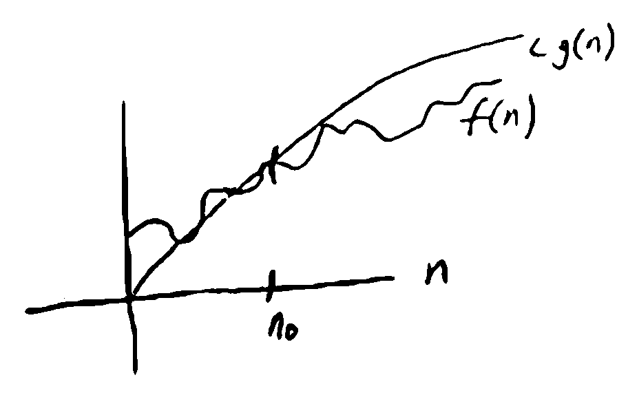
f is asymptotically bounded above by some multiple of g.
Ex.
\(5n = O(n)\)
\(5n + \log n = O(n)\)
\(n^5 + 3n^2 \neq O(n^4)\) since for any constant c, \(n^5\) is eventually larger than \(cn^4\)
\(n^5 + 3n^2 = O(n^5) = O(n^6)\)
Note
\(O(g)\) gives an upper bound, but not necessarily the tightest such bound.
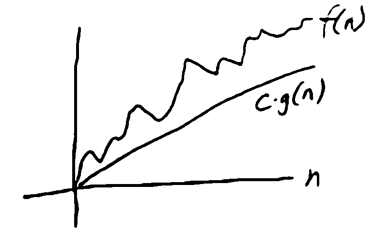
Big-\(\Omega\)
lower bound
\(f(n) = \Omega(g(n))\) if \(\exists c > 0, n_0\) s.t. \(\forall n \geq n_0, f(n) \geq cg(n)\)
Ex.
\(5n = \Omega(n)\)
\(5n+2 = \Omega(n)\)
\(n^2 = \Omega(n)\)
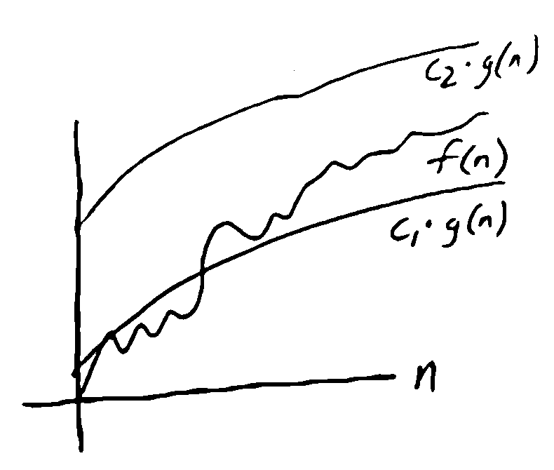
Big-\(\Theta\)
tight bound
\(f(n) = \Theta(g(n))\) if \(f(n) = O(g(n))\) and \(f(n) = \Omega(g(n))\)
if \(f(n) = \Theta(n)\), it is linear time
\(\log n = O(n)\) but \(\neq \Theta(n)\)
\(5n^2+3n = \Theta(n^2)\)
Examples
As example done in class, \(\log_{10}(n)\) is:
- \(\Theta(\log_2(n))\)
Because \(\log_{10}(n)=\frac{\log_2(n)}{\log_2(10)} = c\log_2(n)\) for some c
- NOT \(\Theta(n)\)
need \(\log_{10}(n) \geq cn\) for some \(c > 0\) for some sufficiently large n, which does not hold
so \(\log_{10}(n) \neq \Omega(n)\)
\(O(n^2)\)
- \(\Omega(1)\)
\(\log_{10}(n) \geq c \cdot 1\) for some c
- \(\Theta(2\log_{10}(n))\)
You can set \(c = \frac{1}{2}\)
Some particular growth rates:
- Constant time: \(\Theta(1)\) (not growing with n)
e.g. looking up an element at a given array index
- Logarithmic time: \(\Theta(\log n)\) (base does not matter)
e.g. binary search
- Linear time: \(\Theta(n)\)
e.g. finding the largest element in an unsorted array
Quadratic time: \(\Theta(n^2)\)
- Exponential time: \(\Theta(2^n), \Theta(1.5^n), \Theta(c^n), c > 1\)
e.g. brute-force algorithms