Dynamic Programming
Fundamental idea: write the optimal solution to a problem in terms of optimal solutions to smaller subproblems.
When this is possible, the problem is said to have optimal substructure)
When you can do this, you get a recursive algorithm as in divide/conquer. The difference is that usually the subproblems overlap.
Weighted Interval Solving Problem
Like ISP from earlier, we have n requests for a resource with starting and finishing times, but now each request has a value \(v_i\). We want to maximize the total value of granted requests.
Goal: Find a subset S of requests which is compatible and maximixes \(\sum_{i \in S} v_i\).
Let’s sort the requests by finishing time, so request 1 finishes first, etc.
To use dynamic programming, we need to write an optimal solution in terms of optimal solutions of subproblems. Note that an optimal solution O either includes the last request n or doesn’t.
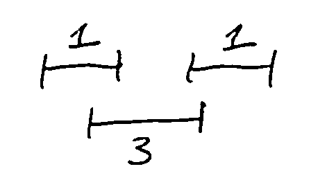
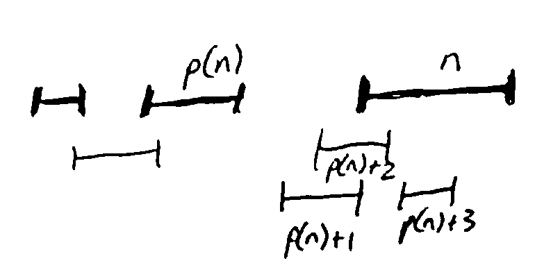
If \(n \in O\), then O doesn’t contain any intervals overlapping with n; let \(p(n)\) be the last interval in the order that doesn’t overlap with n.
Then intervals \(p(n)+1, p(n)+2, ..., n-1\) are excluded from O, but O must contain an optimal solution for intervals \(1, 2, ..., p(n)\).
Note
If there were a better solution for intervals \(1, 2, ..., p(n)\), then we could improve O without introducing any conflicts with n (exchange argument).
If instead \(n\notin O\), then O must be an optimal solution for intervals \(1, 2, ..., n-1\).
Note
If O was not an optimal solution for intervals \(1, 2, ..., n-1\), we could improve O as above.
So, either O is an optimal solution for intervals \(1, ..., p(n)\) plus n, or it is an optimal solution for intervals \(1, ..., n-1\).
If we then let \(M(i)\) be the maximal total value for intervals [1, i], we have:
This recursive equation gives us a recursive algorithm to compute the largest possible total value overall, which is \(M(n)\). We can then read off which intervals to use for an optimal set:
if \(M(n) = M(p(n)) + v_n\), then include interval n
if \(M(n) = M(n-1)\), then exclude interval n
then continue recursively from \(p(n)\) or \(n-1\) respectively.
Runtime
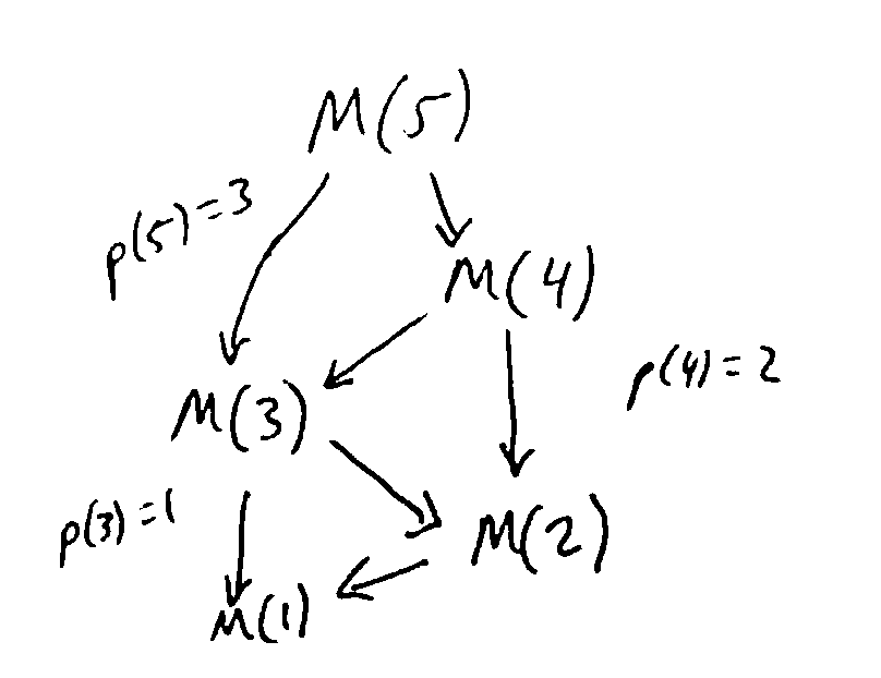
Recursion tree has 2 subproblems, but depth \(\approx n\). So in total, the runtime is \(\approx 2^n\).
But there are only n distinct subproblems: \(M(1), M(2), ..., M(n)\). Our exponentially many calls are just doing the same work over and over again.
Solution: memoization - whenever we solve a subproblem, save its solution in a table; when we need it later, just look it up instead of doing further recursion.
Here, we use a table \(M[1..n]\). Each value is then computed at most once, and work to compute a value is constant, so total runtime will be linear (assuming \(p(i)\) is computed).
Another way to think about memoization: it turns a recursion tree into a DAG by collapsing identical nodes together.
Note
Instead of memoization on a recursive algorithm, we can also eliminate recursion and just compute the “memo table” iteratively in a suitable order.
In the example above, could just compute M[1], M[2], …, M[n] in increasing order: then all subproblems needed to compute M[i] will already have been computed (since M[i] only depends on M[j] with j<i)
M[1] = v1
for i from 2 to n:
    M[i] = max(M[p(i)] + vi, M[i - 1])
TLDR: Dynamic programming = recursive decomposition into subproblems + memoization
Design
Main steps for designing a dynamic programming algorithm:
Define a notion of subproblem; there should only be polynomially-many distinct subproblems
Derive a recursive equation expressing the optimal solution of a subproblem in terms of optimal solutions to “smaller” subproblems
Express the solution to the original problem in terms of one or more subproblems
Work out how to process subproblems “in order” to get an iterative algorithm
Edit Distance
Levenshtein Distance
Distance metric between strings, e.g. “kitten” and “site”.
\(d(s, t)\) = minimum number of character insertions, deletions, or substitutions (replacing a single character with another) needed to turn s into t.
Ex:
kitten
sitten
siten
site
This is the shortest sequence of transformations, so \(d(kitten, site) = 3\). Very useful for approximate string matching, e.g. spell checking, OCR, DNA sequence alignment (see textbook)
Naive algorithm (checking all strings reachable with 1 op, 2 ops, etc) could take exponential time - let’s improve with dynamic programming.
Problem
Given strings s[1..n] and t[1..m], compute \(d(s, t)\). To divide into subproblems, let’s look
at prefixes of s and t.
Let \(D(i, j)\) be the edit distance between s[1..i] and t[1..j]. We ultimately want to compute
\(D(n, m)\).
Let’s find a recursive equation for \(D(i, j)\). Suppose we had an optimal sequence of operations transforming
s[1..i] into t[1..j]. Without loss of generality, we can assume the operations proceed from left to right;
then can view the sequence as an “edit transcript” saying for each character of s what operation(s) to perform,
if any.
Ex: (S = sub, I = insert, D = delete, M = noop)
kitten -(sub k)> sitten -(del t)> siten -(del n)> site

transcript: SMMDMD
Solution
Look at the last operation in the transcript. Several possibilities:
If I, the sequence is an optimal seq. turning
s[1..i]intot[1..j-1]followed by the insertion oft[j], so \(D(i, j) = D(i, j-1)+1\).If D, the seq. is an optimal one turning
s[1..i-1]intot[1..j], followed by deletings[i], so \(D(i, j) = D(i-1, j) + 1\).If S, the seq. is an optimal one turning
s[1..i-1]intot[1..j-1], followed by turnings[i]intot[j], so \(D(i, j) = D(i-1, j-1) + 1\).If M, the seq. is an optimal one turning
s[1..i-1]intot[1..j-1], so \(D(i, j) = D(i-1, j-1)\).
The optimal sequence will take whichever option yields the smallest value of D, so we have
Note
For the base cases, we can use a sequence of insertions/deletions to get from an empty string to another (or vice versa).
Runtime
How long does the recursive algorithm with memoization take to compute \(D(n, m)\)?
Total number of distinct subproblems: \(\Theta(nm)\)
Time for each subproblem: \(\Theta(1)\) (only look at a constant number of previously computed values)
So the total runtime is \(\Theta(nm)\).
Note
The memo table takes \(\Theta(nm)\) memory, but recursion only depends on current and previous value of j, so it is enough to save only the current and previous row of the table.
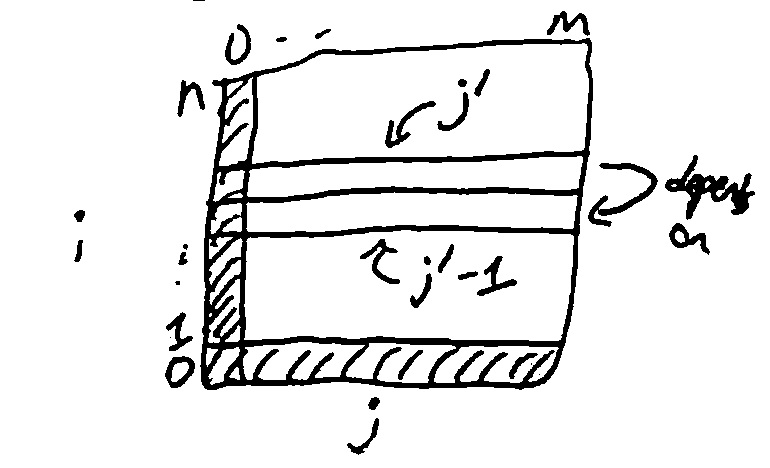
This reduces the memory needed to \(\Theta(m)\).
Bellman-Ford Algorithm
single-source shortest paths with negative weights
Note
If there is a cycle with negative weight (a “negative cycle”), no shortest path may exist.
The BF algorithm can detect this.
Idea
Compute distance \(d(v)\) to each vertex v from source s by dynamic programming.
Note that this is similar to the shortest-path algorithm for DAGs. However, a naive attempt won’t work since the graph can have cycles, which would lead to infinite recursion when trying to compute \(d(v)\).
To fix this problem, we introduce an auxiliary variable in our definition of the subproblems. Here, given source vertex s, let \(D(v, i)\) be the length of the shortest path from s to v using at most i edges. This prevents infinite recursion since we’ll express \(D(v, i)\) in terms of D for smaller values of i.
Solution
Lemma: If there are no negative cycles, the shortest path from s to v passes through each vertex at most once, so \(d(v) = D(v, n-1)\).
To get a recursion for \(D(v, i)\), consider a shortest path from s to v using at most i edges: either it has exactly i edges, or \(\leq i-1\) edges.
If \(\leq i-1\) edges, then \(D(v, i) = D(v, i-1)\)
If exactly i edges, call the last edge \((u, v)\); then we have \(D(v, i) = D(u, i-1) + w(u, v)\).
So, minimizing over all possible cases (including the choice of u):
Now we can compute \(D(t, n-1)\) to get the distance \(d(t)\) using this formula using memoization as usual.
Runtime
Total number of distinct subproblems: n choices for v and n choices for i = \(\Theta(n^2)\)
Notice for each subproblem, we iterate over all incoming edges to v. So for each i, only need to consider each edge exactly once.
Therefore, the total runtime is \(\Theta(nm)\).