Divide-and-Conquer Algorithms
general paradigm used by many algorithms
Divide the problem into subproblems
Conquer (solve) each subproblem with a recursive call
Combine the subproblem solution into an overall solution
This approach is helpful when it isn’t clear how to solve a large problem directly, but you can rewrite it in terms of smaller problems. Coming up with a way to divide/conquer may be easier than solving the whole problem.
Mergesort
e.g. Mergesort: sort a list by recursively sorting two halves - the hard part is merging two sorted lists.
define merge(B, C):

B = [3, 5, 5, 7]  # example data
C = [1, 4, 6]
D = []

look at the first element of each list
pop the smaller and append it to D (or use a pointer to track where in each list you are, etc)

B = [3, 5, 5, 7]
C = [4, 6]
D = [1]

repeat until at least one list is empty

B = [5, 5, 7]
C = [4, 6]
D = [1, 3]

B = [5, 5, 7]
C = [6]
D = [1, 3, 4]

B = [5, 7]
C = [6]
D = [1, 3, 4, 5]

B = [7]
C = [6]
D = [1, 3, 4, 5, 5]

B = [7]
C = []
D = [1, 3, 4, 5, 5, 6]

append the rest of the non-empty list to D
The runtime of the merge operation is linear, i.e. \(\Theta(|B|+|C|)\)
Now we can define mergesort:
def mergesort(A[0..n-1]):
    if n <= 1:
        return A
    mid = floor(n/2)
    left = mergesort(A[0..mid-1])
    right = mergesort(A[mid..n-1])
    return merge(left, right)
The runtime is covered in section (a/n: I didn’t attend, but it’s \(\Theta(n \log n)\)).
Proving Mergesort
How do we prove its correctness? For D/C, induction - assume the recursive calls are correct, and prove correctness given that.
Need to prove that for any list A[0..n-1], mergesort(A) is a sorted permutation of A. Prove by (strong)
induction on n.
- Base Case: \(n \leq 1\)
Then
mergesort(A) = Abut A is already sorted.
- Inductive Case: Take any \(n > 1\), and assume the inductive hypothesis holds for all \(k < n\).
Then \(m = \lfloor n/2 \rfloor < n\)
the length of the left half is \(m\)
the length of the right half is \((n-1)-m+1=n-m=n-\lfloor n/2 \rfloor=\lceil n/2 \rceil < n\)
so
B = mergesort(A[0..m-1])is a sorted permutation ofA(by IH)similarly,
C = mergesort(A[m..n-1])is a sorted permutation ofAsince B and C are sorted, by correctness of
merge(), D is a sorted permutation of B concatenated with Csince B is a permutation of the
A[0..m-1]and C is a permutation ofA[m..n-1], D is a permutation ofA[0..n-1]
Designing
Two questions:
How do you divide the problem into subproblems?
How do you combine the subproblem solutions to get an overall solution?
Integer Multiplication
Given integers x, y, compute x * y.
Note
On a RAM machine, you can only multiply numbers in constant time if they fit in registers; otherwise you need an algorithm.
Elementary Multiplication
    37
x  114
------
   148
   370
+ 3700
------
  4218
If x and y have n digits each, how long does this algorithm take? Each iteration takes linear time, and there are linearly-many iterations, so \(\Theta(n^2)\) in total.
Divide-and-Conquer
Simple idea: split the digits in half, e.g. \(4216 = 42 * 10^2 + 16\)
In general, given an \(\leq n\)-digit integer x, \(x = x_1*10^{n/2}+x_0\) (assuming n is a power of 2).
Likewise, we can write \(y = y_1*10^{n/2}+y_0\).
Then:
This results in 4 multiplications of \(n/2\)-digit numbers: do these recursively. The multiplications by \(10^n\) are just adding zeros, and the additions can be done in linear time.
So, as there are 4 recursive calls, we have:
By the master theorem, this results in \(T(n) = \Theta(n^2)\) - which is not faster than the naive algorithm.
Gotta Go Fast
Let’s look at
Then \(x_1y_0 + x_0y_1 = z - x_1y_1 - x_0y_0\).
So with only 3 multiplications, we can get all 3 terms we need for the algorithm:
\(x_1y_1\)
\(x_0y_0\)
\((x_1+x_0)(y_1+y_0) = z\)
and you can substitute into the earlier equation \(xy = x_1y_1*10^n + (z - x_1y_1 - x_0y_0)*10^{n/2} + x_0y_0\) to obtain the product.
This results in a speedup at every recursive call, which adds up.
Now our recurrence is \(T(n) = 3T(n/2) + \Theta(n)\), which by the master theorem results in \(T(n) = \Theta(n^{\log_2 3}) \approx \Theta(n^{1.58})\)
This is faster than the naive algorithm!
Gotta Go Faster
There is, in fact, a faster algorithm that runs in \(O(n \log n \log \log n)\) based on the Fast Fourier Transform - but it only really starts being faster when you reach n in the thousands.
This algorithm is not covered in this class - see AD 5.6 or CLRS 30.

Well.
In 2019, a \(O(n \log n)\) algorithm was found, but the point at which it becomes faster is only for astronomically large n.
Closest Pair
find the closest pair of points in the plane
Given a set of n points in the plane, find the pair of points which are closest together.
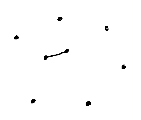
Naive algorithm: Check all possible pairs, and take the pair with least distance (\(\Theta(n^2)\)).
D/C Algorithm
Divide: take the left and right halves of the points
In order to do this efficiently, start by sorting the points by their x-coordinate
Then the first half of the sorted array has the leftmost n/2 points, and the second half the n/2 rightmost
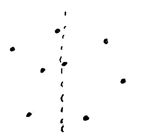
Then, use recursive calls to find the closest pair of points on the left side and right side.
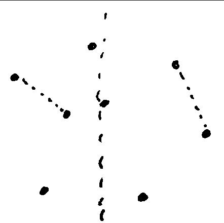
But, we haven’t considered pairs where one point is in the left half and the other is in the right half.
If we simply checked all pairs such that one point was on the left and one was on the right, we’d still end up with \(\Theta(n^2)\). Instead, we filter out many pairs which cannot be the closest.
Idea: If the recursive calls find pairs at distances \(\delta_L, \delta_R\) from each other on the left and right sides respectively, then we can ignore all points that are further than \(\delta = \min(\delta_L, \delta_R)\) from the dividing line.
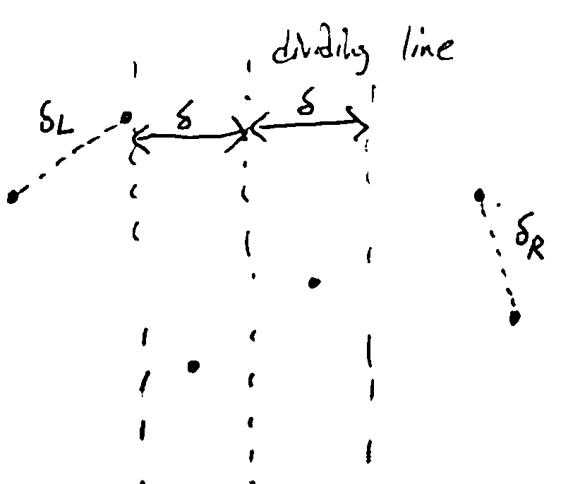
Now, we can consider only the points in the “tube”. We can find the points inside this tube in linear time, since the points are sorted by x-coord already.
Idea 2: On both the left and right, no pairs are closer than \(\delta\) together. By drawing boxes of size \(\delta/2 \times \delta/2\), there is at most one point in each box.
Then, any point on the left can only be within \(\delta\) of a finite number of boxes on the right.
So, we’ll take the points in the left and right halves of the tube, and consider them in y-coordinate order (sort by y at beginning of algorithm so this is linear). For each point, compute its distance to the next 15 points in the order, keeping track of the closest pair found so far.
Note
Why 15? Because we drew these boxes, if a point is to be within \(\delta\) of the considered point, it must be within one of the next 15 boxes. We check 15 points for the worst case scenario, if every single box is full.
If we find a pair that is closer than \(\delta\), return that pair; otherwise return the pair at distance \(\delta\).
Runtime
- First, we sort by x and y at the beginning: \(2n\log n = \Theta(n \log n)\)
This doesn’t affect the recurrence, since it only happens once, not at each level of recursion.
Recursive part: 2 calls for the left and right: \(2T(n/2)\)
Then a linear amount of work to filter out points not in the tube: \(\Theta(n)\)
Then linear amount of work again, comparing each point to the 15 next points: \(15n = \Theta(n)\)
So we have \(T(n)=2T(n/2)+\Theta(n)\), which is \(T(n)=\Theta(n \log n)\).